Old NLP Paper Reviews
Premise
This is part of an ongoing series where I revisit influential papers in NLP. Each post will briefly summarize the core ideas, highlight what I found interesting (or confusing), and sometimes include small experiments. The goal isn’t to be exhaustive.
Attention is All You need (Vaswani et al., 2017)
Written in Oct 30, 2025
Many people consider this the landmark paper that ignited the Transformer revolution.
\[\text{Attention}(Q, K, V) = \text{softmax}\left(\frac{QK^T}{\sqrt{d_k}}\right)V\]This is the mechanism that started it all. Much have changed since then: I will focus on what I found interesting when reading the paper again.
About Attention Mechanism
The two most commonly used attention functions are additive attention [2], and dot-product (multiplicative) attention. Dot-product attention is identical to our algorithm, except for the scaling factor of \(\sqrt{d_k}\). Additive attention computes the compatibility function using a feed-forward network with a single hidden layer. While the two are similar in theoretical complexity, dot-product attention is much faster and more space-efficient in practice, since it can be implemented using highly optimized matrix multiplication code.
This shows that the idea of attention itself was not new. Previous paper also introduced attention mechanism. It was used as a middle layer connecting encoder and decoder RNNs. The novelty of this paper was showing that attention mechanism alone can be used to replace RNNs.
That said, I think that the title “Attention Is All You Need” is slightly misleading. When I first read the paper, I assumed attention parameters dominated model size. In reality, most parameters come from the feed forward layers (FFN) within each attention block. Many LLMs use 4 times dimension expansion in the FFN layer, with some recent MoE models even more aggressively expanding the FFN dimensions. (95%+ of parameters in case of OpenAI OSS models).
| Component | Complexity | Parameter Share |
|---|---|---|
| Attention | (O(n^2 d)) | ~30 % |
| FFN (MLP) | (O(n d^2)) | ~70 % |
Parameter share numbers are estimates if we use 4x dimension expansion in FFN layers with standard attention.
Furthermore, works have focused on the calculation of the attention weights, which is \((O(n^2 \cdot d))\). However, the feed-forward layers also have complexity of \((O(n \cdot d^2))\), Since in the earlier days of transformers, \(d\) was often larger than \(n\), the feed-forward layers were more computationally expensive on simple tasks.
About Positional Embeddings
The paper introduced sinusodial positional embedding. That is,
\[\text{PE}_{(pos, 2i)} = \sin\left(\frac{pos}{10000^{2i/d_{model}}}\right)\] \[\text{PE}_{(pos, 2i+1)} = \cos\left(\frac{pos}{10000^{2i/d_{model}}}\right)\]where pos is the position and i is the dimension. That is, each dimension of the positional encoding corresponds to a sinusoid. The wavelengths form a geometric progression from 2π to 10000 · 2π. We chose this function because we hypothesized it would allow the model to easily learn to attend by relative positions, since for any fixed offset k, \(PE_{pos+k}\) can be represented as a linear function of \(PE_{pos}\)
So what does this mean? Simply, put, we can design a rotational matrix \(\mathbf{R}^k\) such that
\[\mathbf{R}^k \cdot PE_{pos} = PE_{pos+k}\]Such rotational matrix can be created by the following block diagonal matrix.
\[R_i^k = \begin{pmatrix}\cos k / 10000^{2i/ d_{model}} & -\sin k / 10000^{2i/ d_{model}}\\ \sin k / 10000^{2i/ d_{model}}& \cos k / 10000^{2i/ d_{model}}\end{pmatrix}\] \[\mathbf{R}^k = \begin{pmatrix} R_0 & & & \\ & R_1 & & \\ & & \ddots & \\ & & & R_{d_{model}/2} \end{pmatrix}.\]This also means position embedding difference between two tokens are determined by its relative distance.
I personally find this formulation elegant but slightly lacking. We can express this as:
\[\mathbf{R}^k \times PE_{pos} + emb = PE_{pos + k} + emb\]However, the attention mechanism is not additive. It uses dot product attention, and capturing additive positional difference seems unaligned to me. I would consider the following to be more intutive.
\[\mathbf{F}(P(x,pos), k) = P(x, pos + k)\]\(P(x, pos)\) here is a function that encodes the position \(pos\) and token embedding \(x\) together. A position encoding should have some function \(\mathbf{F}\) that allows shifting the position by \(k\) when applied. This too, however, is counte to the linear additive nature of the transformers. Thus one might want a position embedding that keeps the latent representation additive while making attention mechanism rotational. Rotary Position Embeddings (RoPE) satisfy this property.
The paper also notes that replacing the sinusoidal embedding with a learnable one barely affects performance.
Simple Experiments
- Sinusodial Embedding vs Learnable.
- Additive (Bahdanau-style) vs Dot product attention.
For the base transformer implementation, I used the Andrej Karpathy’s minGPT and evaluated based on the perplexity of the Shakespeare dataset. The code can be found here.
There was a minor difficulty in implementing the Bahdanau Attention. The original attention mechanism in the paper (Which connects encoder with decoder) uses the following
\[\alpha_{ij} = \frac{\exp(e_{ij})}{\sum_{k=1}^{T_x} \exp(e_{ik})} \quad \\ e_{ij} = v_a^T \tanh(W_a s_{i - 1} + U_a h_j)\]where \(v_a \in \mathbb{R}^n\), \(W_a \in \mathbb{R}^{n \times m}\), \(U_a \in \mathbb{R}^{n \times 2m}\). More detail can be found in the original paper.
To fit this implementation to Transformers, I modified the equation a bit.
\[e_{ij} = vx_i\tanh(W_q x_i + W_k x_j)\]Let head size be denoted \(h\). Then, we have \(v \in \mathbb{R}^{h}\), \(W_q \in \mathbb{R}^{h \times h}\), \(W_k \in \mathbb{R}^{h \times h}\).
Notice that \(v\) here is a 1d vector instead of a matrix as in transformer. This was a design choice to be closer to the original Bahdanau attention. The \(q,k\) vectors are same as the original transformer.
But this approach takes up too much memory in parallel computation. We need to materialize matrix of (B, T, T, h) tensor to parallelize adding the \(q,k\) vectors. So I used an alternative implementation.
\[e_{ij} = v(\tanh(W_q x_i)) + v(\tanh(W_k x_j))\]This way, we do not need to materialize the full (B, T, T, h) tensor. The two implemtations are not equivalent, but I think this is a reasonable approximation.
Results
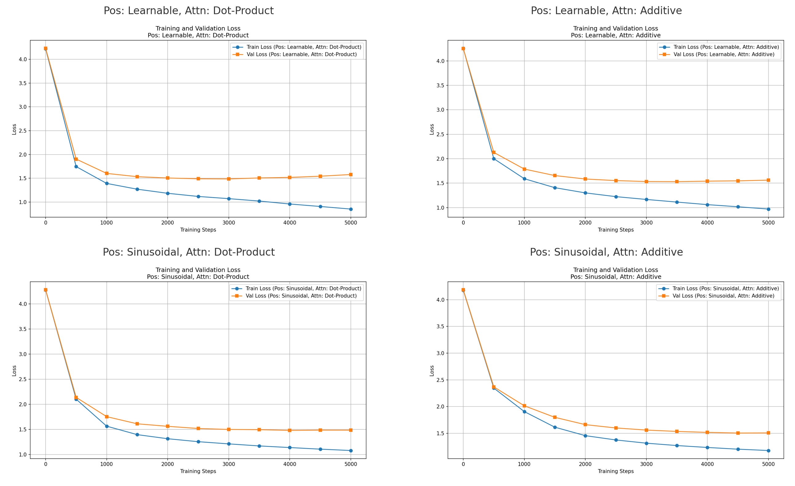
All models produced similar perplexity curves — confirming that both learnable vs. sinusoidal embeddings and additive vs. dot-product attention behave comparably on small datasets.
Takeaways
- Attention wasn’t new — the innovation was using attention-based blocks.
- FFN layers dominate parameters, and sometimes, compute — attention is important, but not the whole story.
- Sinusoidal embeddings are fixed position embedding which allow relative position encoding via rotation.
Chain of Thought Prompting Elicits Reasoning in Large Language Models (Wei et al., 2022)
Written on Nov 1, 2025
This paper is widely regarded as the beginning of the “reasoning” era in large language models. Chain-of-Thought (CoT) prompting demonstrated that simply adding step-by-step reasoning in prompts dramatically improves performance on arithmetic, commonsense, and symbolic tasks. CoT directly inspired later frameworks such as ReAct (reasoning + acting) and motivated the development of models explicitly trained on reasoning traces.
Building on this, researchers began using reinforcement learning on reasoning processes to create “thinking” or “reasoning” models—systems that learn to generate intermediate reasoning steps before producing a final answer. OpenAI’s o1 was one of the first marketed LLMs to incorporate these ideas.
Core Idea
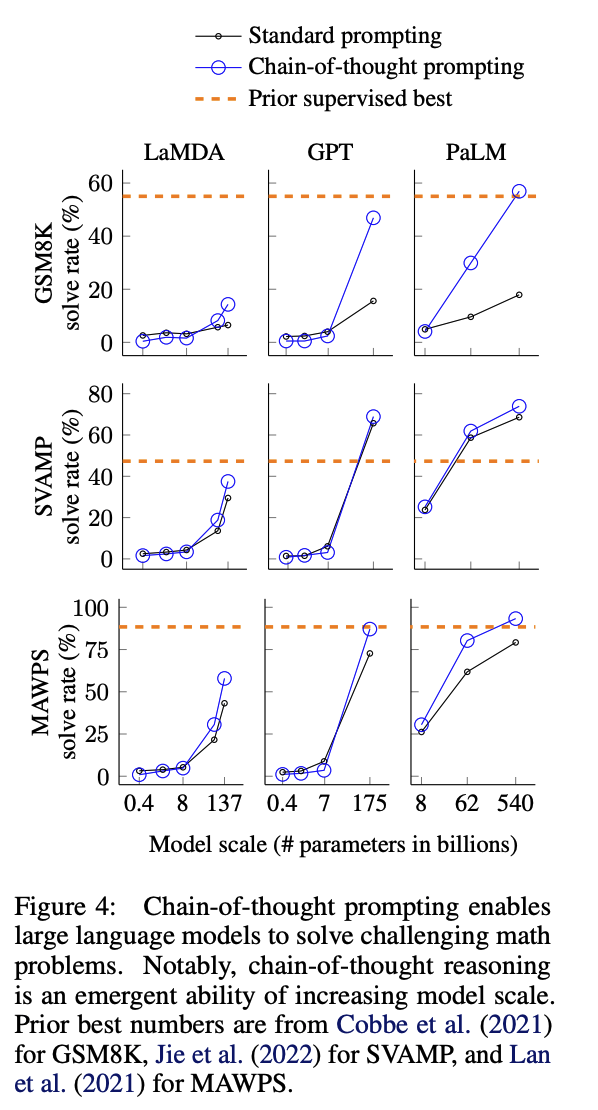
Prompting LLMs with few-shot step-by-step reasoning examples significantly improves performance on complex reasoning tasks. The authors showed that this works on arithmetic, commonsense, and symbolic reasoning benchmarks.
This method worked better than standard few-shot prompting, especially as the model size increased. Models with size less than 10B often degraded in performance with CoT while larger models such as GPT-3 and PaLM 540B showed improved performance.
The authors hypothesize that the ability to reason might be an emergent behavior with model size.
Additional Tests
In order to see which aspect of the CoT prompting helped, the authors designed several prompt variants.
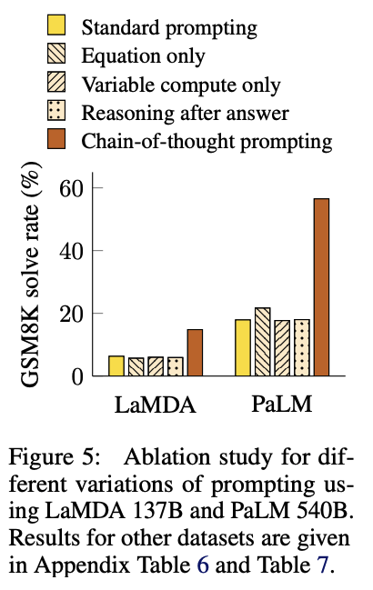
For GSM8k, they provided models with
- Standard Prompting (few-shot)
- Equations only, no reasoning steps.
- Variable compute only, where the llm was given sequence of dots (…) equal to the original CoT.
- Chain of Thought After the Answer.
- Chain of Thought Before the Answer (original CoT).
The results show that only the original CoT prompting significantly improves performance. This suggests that the step-by-step reasoning process itself is crucial.
Personal Thoughts
I wonder if their claim about model size and emergence still holds true in 2025. We have different training pipelines: training data, model architecture and SFT -> RL is different from 2020. One major problem is that the comparison is not an apples to apples comparison, as recent training data often includes the reasoning rollout. I do think that retesting the claim with curated data, MoE model would be interesting.
Since CoT and its variants are popular methods for prompting, I assumed that some organization would have kept a record of the results. With this, I would have been able to compare the accuracy increase claims on newer models. I couldn’t find it, and decided to test on smaller models.
After being unhappy on my own CoT prompts and answer extractor, I used ElutherAI’s LM Evaluation Harness to prompt and evalute LLM responses from GSM8k. As a side note, I think the uncentralized evaluation for LLMs is quite problematic: Some of the small improvements can be due to a more broad regex extractor, or from the randomness of the evaluative LLMs.
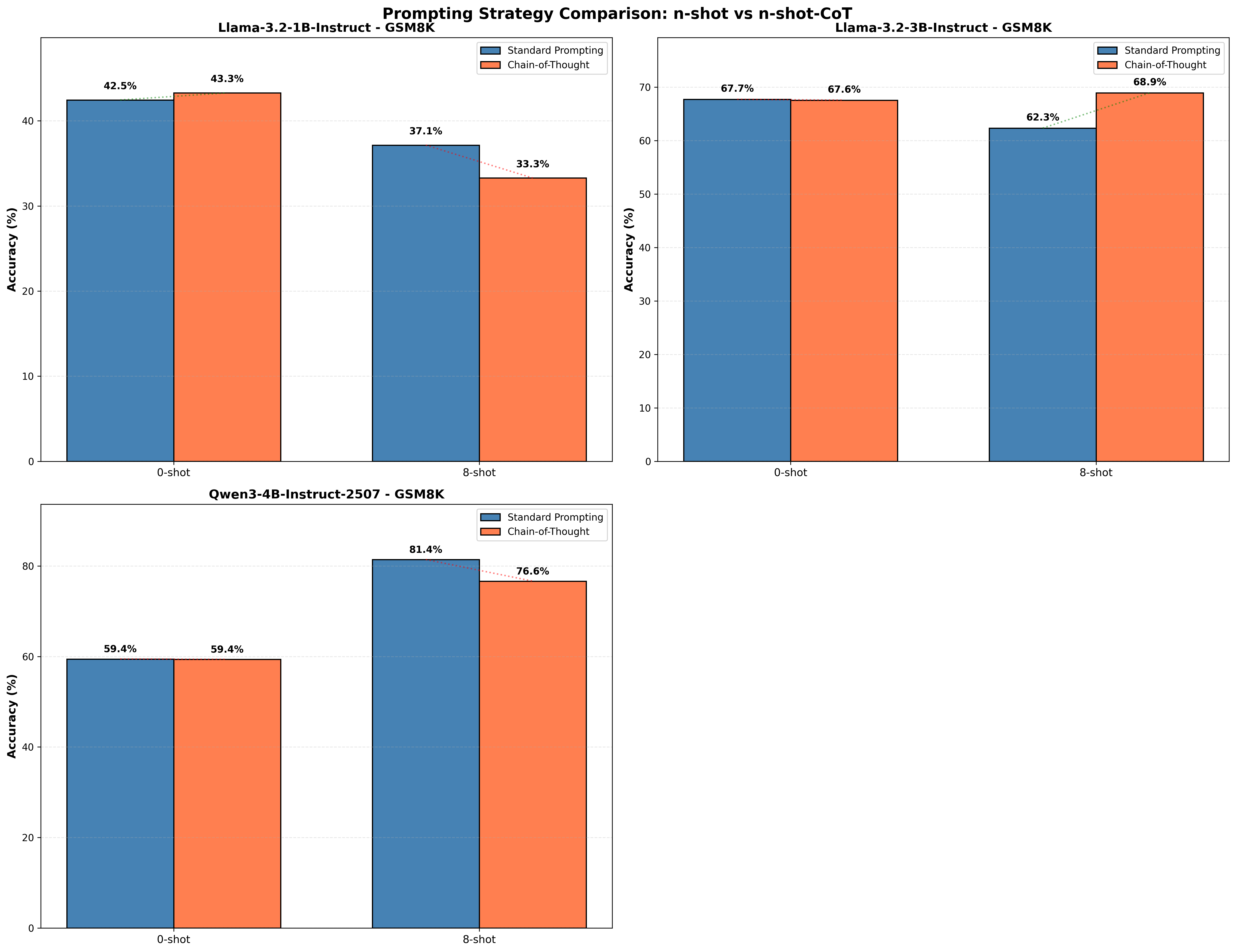
The 0-shot Chain of Thought version here isn’t the popular Zero shot CoT (Often referred as just CoT in some context) but prompt with zero examplars. The left bars could be seen as standard prompting with 0-shot standard and Chain-of-Thought prompting can be seen as directly asking the question without any context. (The difference between the two should be the variance).
We see that CoT prompting hurts performance for Llama 3.2 1B model, while slightly improving Llama 3.2 3B and Qwen3 4B model. Furthermore, we see that standard prompting outperform the CoT version when prompted with the Llama 3.2 1B and Qwen3 4B models. The model performance with and without CoT is model dependent in this experiment, and probably is dataset dependent.
Closing Remarks
Chain of Thought had a great impact on LLMs, affecting the prompting strategies and fine tuning pipelines. This can be directly seen in LLMs. Earlier tended to output only the final answer for mathematical and reasoning tasks. Now, even small models tend to explain their steps and output the final answers.
This is an instance where human understanding of the world have improved ML model. Prompting and training models on how humans think resulted in a better model performance, counter to the spirit of bitter lesson, which argues that progress in AI comes from building system that learn on that own, not from encoding what we know.
Maybe Chain of Thought style training will hit a wall in the near future. Of course, there are alternatives such as teaching the models to reason in latent space.
ROFORMER: ENHANCED TRANSFORMER WITH ROTARY POSITION EMBEDDING
Written in Nov 21, 2025
Rotary Positional Embedding (RoPE) is practically used in all modern LLMs. Llama, Qwen, and even the recent Olmo3 all use it. This paper introduced this embedding.
What is RoPE?
Simply put, instead of adding a sinusodial position embedding to the \(x\) vector, as done in the original transformer paper, The rotation is applied to the \(q,k\) vectors.
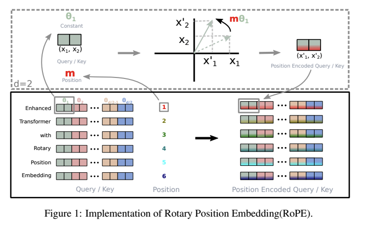
This creates some interesting properties.
Theoretical Explanation of RoPE
Section 3.4 explains the validity of the RoPE. It requires the unnormalized attention values \(q_m k_n\) to
- Be same if the distance (\(n-m\)) are the same.
- Be the original values of \(q,k\) if \(m, n\) are zero.
The paper shows that their formulation of Rotary Position embedding satisfies this property.
They also show an upper bound for this value to be \(\left( \max_i \lvert h_{i+1} - h_i \rvert \right) \sum_{i=0}^{\frac{d}{2}-1} \lvert S_{i+1} \rvert\), showing that the dot product reduces with more distance.
Paper’s Performance Results of RoPE
The paper shows effectiveness of RoPE by comparing its performance with sinnusodial position embedding in the original attention paper. The result is as follows.
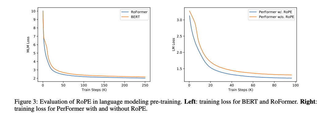
The right graph compares RoFormer to a standard BERT baselline (using learned absolute embedding). The graph on the left uses PerFormer, a linear attention.
This result is the one that surprised me the most when reading this paper. I expected the loss to be more drastic, as RoPE is currently used in virtually all of Transformers. The results show a measly increase in performance, an increase where in some eyes, might be just because of luck instead of actual improvement. Same can be said for result on downstream tasks, where learned positional embedding perform better than RoFormer (Their postional embedded transformer) in some tasks.
Additional Experiment.
The paper argues that their method have a long distance decay. They argue that by proving that the expression is bounded above by \(\left( \max_i \lvert h_{i+1} - h_i \rvert \right) \sum_{i=0}^{\frac{d}{2}-1} \lvert S_{i+1} \rvert\). However, their graph only lasts up to around position ~260. What happens for longer sequencs? Does the relative upper bound go to zero, or does it stay stable? In some chance, the upper bound can increase after some time.
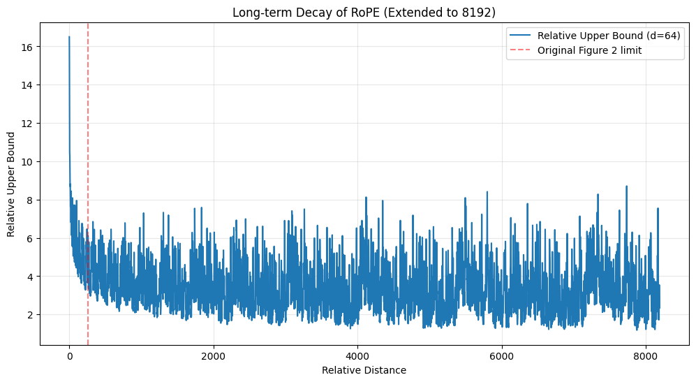
The graph suggest that the upper bounda stays stable (for d = 64) from 2 to 6 for 2000+ positions.
Personal Thoughts
When I decided to read this paper, I was expecting a monumental increase in performance, or a quality, such as decreased performance degradation over time, for Rotary Position Embedding. In fact, there should be a reason behind why all transformers use RoPE. However, this wasn’t the case. The results showed that their embedding is extrapolatable to longer distance, but didn’t do a short context learning -> long context training, or show a drastic increase in performance compared to previous embedding mechanism.
Enjoy Reading This Article?
Here are some more articles you might like to read next: