Random Cosine Similarity Distribution

Problem with Uninterpretable Scores

In machine learning, many scores or values are difficult to interpret in siolation. For example, take BERTScore. While we know that higher scores indicate greater similarity, the raw values lack intuitive meaning. Is the difference between 0.7 and 0.8 comparable to the difference between 0.8 and 0.9? What constitutes a “good” BERTScore?

Furthermore, in Retrieval Augumented Generation (RAG) systems, consine similarity between the query and document embeddings are often used to determine relevant documents. However, the cosine similarity itself is not interpretable. A cosine similarity of 0.7 might seem reasonable, but how much better is 0.8? Without context, these numbers are difficult to assess.

More fundamentally, matrix multiplication is simply a parallelized version of a dot product, which is scaled cosine similarity. I noticed that I lack the intuition of cosine similarity values in high dimensional spaces. This motivated me to investigate the distribution of cosine similarities between random vectors in a unit hypersphere.

Experiment Starting with 2D

I To build intuition, I started with a simple 2D unit circle. Before you read further, try to guess what the cosine similarity distribution would look like.

import math
import random
import matplotlib.pyplot as plt
def get_random_point_on_circle():
    angle = random.uniform(0, 2 * math.pi)
    x = math.cos(angle)
    y = math.sin(angle)
    return (x, y)

random_points = [get_random_point_on_circle() for _ in range(10000)]

first_item = random_points[0]
cosine_similarities = []
for i in range(1, len(random_points)):
    dot_product = first_item[0] * random_points[i][0] + first_item[1] * random_points[i][1]
    cosine_similarities.append(dot_product)

plt.hist(cosine_similarities, bins=50)
plt.title("Histogram of Cosine Similarities of Unit Vectors in 2D")
plt.xlabel("Cosine Similarity")
plt.ylabel("Frequency")
plt.show()

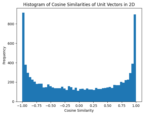
The histogram looks like below.

Cosine similarities are more likely to be around extreme values of -1 and 1 and less likely to be around 0! This is quite counter-intuitive. I asked three people about this and all three guessed that the distribution would be uniform.

Understanding the 2D Distribution

Why does this happen? Let’s build geometric intuition.

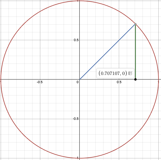
We can fix the first vector to \((1,0)\) without loss of generality. If we look at the first quadrant of the unit circle, we see that \(x = y\) line bisects the circumference of the quadrant. However, the cosine similarity of the midpoint is \(\frac{\sqrt{2}}{2} \approx 0.707\). Since cosine of 90 degrees is 0, and cosine of 0 degrees is 1, we expect to see the same number of points with cosine similarity between 0 and 0.707 and cosine similarity between 0.707 and 1. This explains why we see more points around extreme values.

Another way to look at it would be to look at the slope. The slope of the circle at \((1,0)\) is perpendicular, while at \((0,1)\) it is horizontal. Thus a change in angle near \((1,0)\) results in a small change in cosine similarity, while a change in angle near \((0,1)\) results in a large change in cosine similarity.

Higher Dimensions

For higher dimensions, manually coding the angular rotations becomes error-prone. there exists an elegant approach which leverages the properties of the multivariate normal distribution: sample from a standard normal distribution, and then normalize. The reason is that multivariate normal distribution has spherically symmetric distribution, so normalizing the sampled vector results in a uniform distribution on the unit hypersphere.

import numpy as np
def random_point_on_unit_sphere(n: int) -> np.ndarray:
    point = np.random.randn(n)
    point = point / np.linalg.norm(point)

    return point

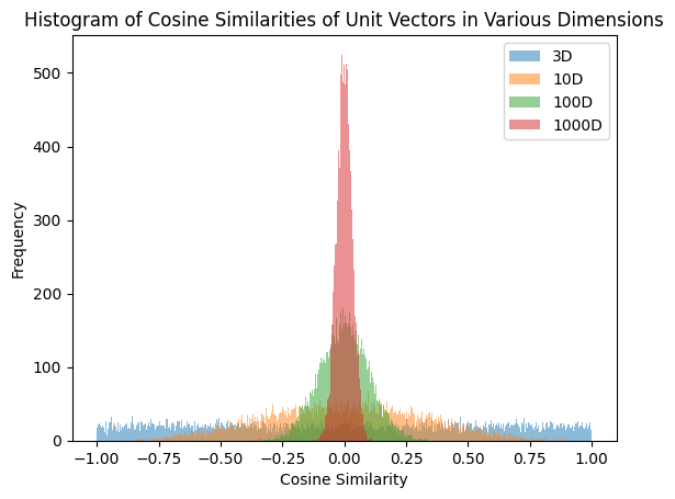
Using this function, I plotted the histogram of cosine similarities in 3D, 10D, 100D, 1000D below.

As dimension increases, the cosine similarities are more concentrated around 0. For 100D, there is no sample with cosine similarity greater than .3 among 10,000 samples.

Another interesting observation is that in 3 dimension, the distribution looks uniform. GPT5 shows that it is indeed uniform in 3D case. In fact, it showed that the distribution of the cosine similarity of dimension \(d\) follows a Beta distribution with parameters \((\frac{d-1}{2}, \frac{d-1}{2})\) link.

Implications for Embeddings

Text embedding models often assign cosine similarities above 0.7 to similar documents. In high-dimensional spaces (common embeddings use 384, 768, or 1536 dimensions), such high cosine similarities are extremely rare between random vectors. This means that semantically similar texts must have embeddings that are highly aligned in the embedding space, far from the random baseline.